How open models actually learn new abilities in 2026 — Part 1: the on-policy-distillation shift

If you have watched open-weight model releases over the last year, you have seen the pre-training recipe converge (everyone scrapes the web, filters it, and predicts the next token) while the post-training recipe, the part that turns a raw pre-trained model into something you would actually talk to, stayed messy and secretive. This two-part series is about one specific thing that changed in that messy part in 2026, and it is a change worth understanding whether you train models yourself or just want to know how the models you use got built.

Here is the whole story in one sentence: a growing number of frontier open labs have stopped trying to make one model learn everything at once, and instead build many single-capability models and fuse them into one — increasingly with a technique called on-policy distillation. It is not the only way labs still do this, but it is the one that has been spreading fastest. Part 1 (this post) explains what that means from the ground up and why it works, with the real math. Part 2 covers who does it, how their recipes differ, and what it means for the GPUs you rent.

Let me start from zero, because the payoff only lands if the setup is clear.

What post-training even is, and the one hard part

A pre-trained model is a next-token predictor. Post-training is everything you do after that to make it useful: teach it to follow instructions, to reason through a math problem, to write correct code, to use tools. The field has largely agreed on the ingredients. First supervised fine-tuning (SFT): show the model examples of good answers and have it imitate them. Then reinforcement learning (RL), specifically RL with verifiable rewards (RLVR). The name was coined by the Allen Institute for AI's Tülu 3 (arXiv 2411.15124), a method that "only gets a reward if the model's completions are verified to be correct." The GRPO algorithm most of these recipes run on was introduced a few months earlier in DeepSeek's DeepSeekMath (arXiv 2402.03300), and verifiable-reward RL was then popularized at scale by DeepSeek-R1. You let the model try a math problem, check the answer, and reward it when it is right. RLVR is how models got good at things with a checkable answer: "mathematics and precise instruction following," in Tülu 3's words.

Training one capability this way is, by 2026, well understood. The hard part was never one capability. It was combining several.

Picture it concretely. You have used RLVR to build a model that is excellent at competition math. Separately, you built one that is excellent at resolving SWE-bench-style software issues. And a third that follows finicky formatting instructions flawlessly. Each is a specialist. Now your users want one model that does all three well. How do you combine three models into one without the combination being worse than each part?

That question, call it the integration problem, is what the 2026 shift is really about. And the reason it is hard is that the obvious ways to solve it all fail, each in its own way.

The integration problem fails four ways

The MOPD paper from Xiaomi's LLM Core team (arXiv 2606.30406) is the paper that formalizes the technique this series is about, and the source of every ablation number below. It lays out the menu of integration options and where each one breaks. It repays a slow read, because understanding why the alternatives fail is what makes the winning method look inevitable.

Say each specialist was branched from the same starting checkpoint. Here are your options for fusing them:

Parameter merging — average the weights. Just take the numeric weights of the three models and average them, or add up their differences from the base. It is appealing because it is free: no training, done offline in minutes. The problem is that a neural network's weights are not a coordinate system where "halfway between two good models" is itself good. Averaging in weight space is unstable and routinely fails to reproduce what the specialists could do. In the MOPD paper's head-to-head comparison of integration methods, a linear weight-merge scores 0.328 and the smarter "task arithmetic" merge 0.857, both well short of what on-policy distillation reaches (0.937) on the same task. Capability is left on the floor.

Off-policy distillation — imitate the teacher's answers. Have each specialist generate lots of good solutions, pool them, and fine-tune the student to copy them: plain supervised fine-tuning on the teacher's outputs. This gives a dense learning signal (the student gets feedback on every token) which is good. But it has a subtle, fatal flaw called exposure bias. The student only ever trains on the teacher's trajectories, which are not quite trajectories the student would produce itself. At inference time the student inevitably drifts a little, lands in a state the teacher never demonstrated, and, having never been trained on its own mistakes, compounds the error. It learned to imitate a path, not to recover when it steps off it.

Mix-RL — one big joint RL run. Train math, code, and instruction-following together in a single reinforcement-learning job. This keeps learning on-policy (the model learns from its own attempts, fixing exposure bias) and is the 2025 default. But domains interfere. Pushing math accuracy up drags code accuracy down; you tune to fix code and math slips. Practitioners call it the see-saw effect. Worse, it is a single giant coupled job: change one domain's reward function or data mix and you restart the entire run.

Cascade RL — one domain after another. RL on instruction, then on math, then on code, and so on. Also on-policy. But each new stage erodes the earlier ones (the classic catastrophic forgetting) so you are left babysitting a long, fragile run and watching abilities you already paid for decay.

Step back and the pattern is stark. Every option is missing at least one of three properties you want:

• a dense signal (feedback on every token, not one score at the end),
• on-policy learning (the model learns from its own outputs, so it is robust at inference),
• and parallelizable production (you can build the specialists independently, in parallel, without one blocking another).

Table 1 — Five ways to fuse specialists, and where each breaks down. Only on-policy distillation is dense, on-policy, and parallelisable at the same time. Axes from MOPD (arXiv 2606.30406).

Integration method	Dense signal	On-policy	Parallelisable	Failure mode
Parameter merging (weight averaging)	✗	—	✓	weight-space fusion unstable; specialists not reproduced
Off-policy distillation (SFT on teacher answers)	✓	✗	✓	exposure bias / compounding error
Mix-RL (one joint RL run)	✗	✓	✗	see-saw / domain interference
Cascade RL (one domain after another)	✗	✓	✗	catastrophic forgetting
On-policy distillation	✓	✓	✓	—

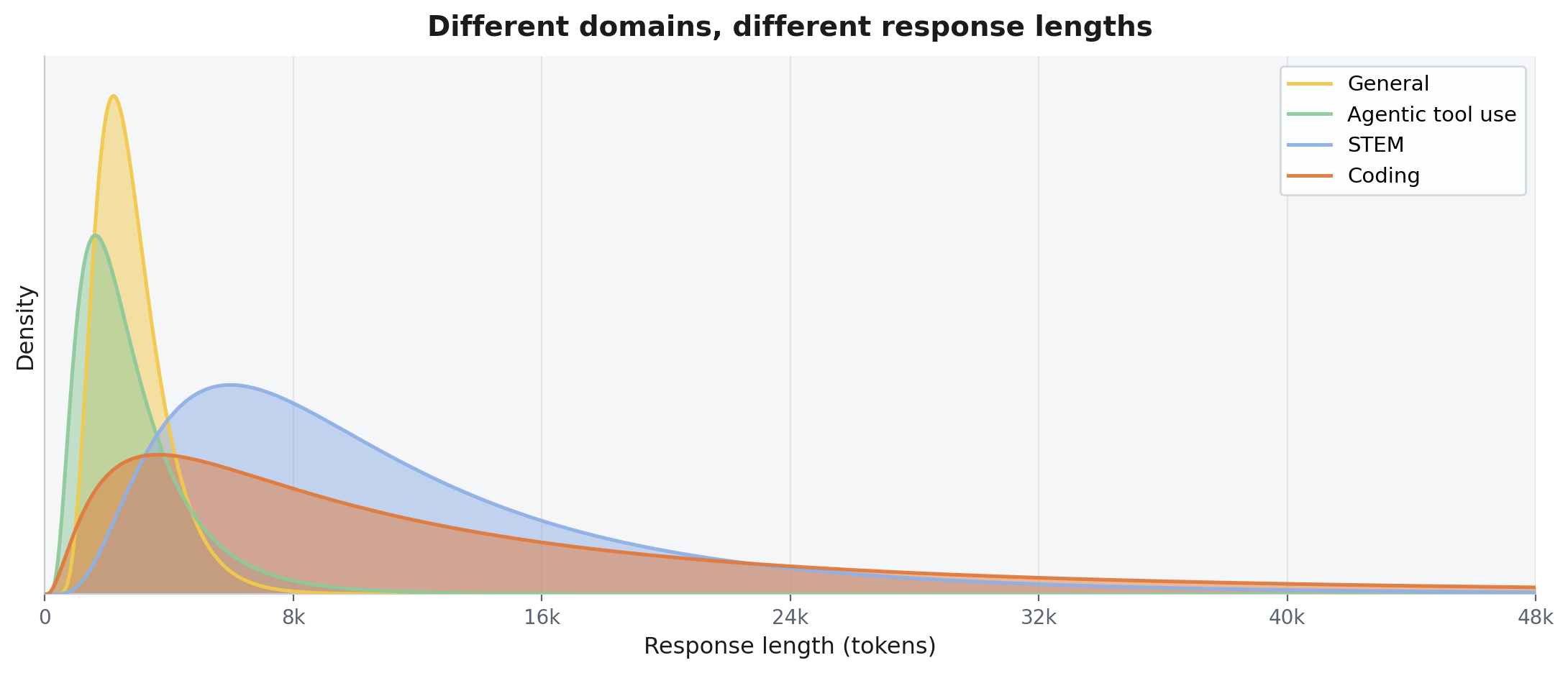
And the interference is not a whiteboard worry: labs measure it. When Meituan built LongCat-Flash-Thinking in 2025, they logged how many tokens their model spent answering in each domain, and the distributions barely overlap: general chat wraps up in a few thousand tokens, while a coding solution can trail out toward fifty thousand (Fig 1). Push all of that through one shared RL run and every gradient step is yanked toward incompatible targets at once. The paper calls the result negative transfer. That is the measured, mechanical reason a single mixed run fights itself.

Parameter merging is dense-ish but off-policy and unstable. Off-policy SFT is dense but off-policy (exposure bias). Mix-RL and cascade RL are on-policy but sparse (one reward per attempt) and not parallelizable: they couple everything together. There is exactly one method that is dense, on-policy, and parallelizable at the same time. That is on-policy distillation, and the rest of this post is about why that combination is not a lucky coincidence but the whole point.

What on-policy distillation actually is

The intuition first. Think about how you would coach someone. Option 2 above (off-policy SFT) is like handing a student a stack of worked solutions and telling them to memorize the style. They learn to reproduce answers that look right, but the moment they face a slightly different problem and take a wrong first step, they are lost, because nobody ever watched them work. On-policy distillation is the opposite. You let the student solve the problem their own way, and an expert looks over their shoulder and grades every single line as they write it: "that step is good, that one is where you went wrong." The student gets detailed feedback on the exact path they actually took.

The mechanism. On-policy distillation was presented as a clean, general recipe by Thinking Machines Lab in October 2025 (the reverse-KL, on-policy idea itself goes back to earlier work like GKD and MiniLLM, ~2023–24). Three steps:

1. The student samples its own trajectory, its own attempt at the prompt.
2. A stronger teacher scores every token of that trajectory. This is the crucial part: the teacher does not generate anything. It runs a single forward pass over the student's already-written tokens and reports, for each position, how probable that token was under the teacher. It is scoring, not decoding, closer to a grader than to a second writer. (This is why, later in Part 2, the teacher turns out to be cheap to serve: forward-only work, no slow token-by-token generation.)
3. The student is updated to make its trajectory more probable under the teacher: formally, by minimizing a per-token reverse KL divergence between student and teacher.

Written out, the objective is a sum, over every token the student produced, of the KL divergence between the student's and teacher's next-token distributions at that position:

The expectation is over the student's own samples (y ∼ π_θ): that is the "on-policy" part. The D_KL(π_θ ‖ π_T) inside is the "distillation" part. That is the entire idea. Everything else is a choice about how to compute that KL and which teacher to point it at.

Why this specific divergence? Here is the layer that trips people up, and it is worth doing correctly. KL divergence is not symmetric (D_KL(p ‖ q) is not the same as D_KL(q ‖ p)) and the direction matters enormously.

Suppose the "true" or teacher distribution p has two separate good answers (two modes) and your student q is simpler and can really only commit to one shape. What does each direction of KL ask the student to do?

• Forward KL, D_KL(p ‖ q), is weighted by p. It punishes the student hardest wherever the teacher puts mass but the student does not. To avoid that penalty the student must put some probability everywhere the teacher does: it becomes mode-covering, smearing itself across both modes and, inevitably, across the empty valley between them. This is exactly what ordinary maximum-likelihood SFT does, and it is why an over-hedged model will sometimes produce a blurred average of two good answers.
• Reverse KL, D_KL(q ‖ p), is weighted by q. It only penalizes the student where the student itself puts mass. The student is free to ignore one of the teacher's modes entirely, as long as wherever it does commit, the teacher agrees. This makes it mode-seeking: it picks one good answer and sharpens.

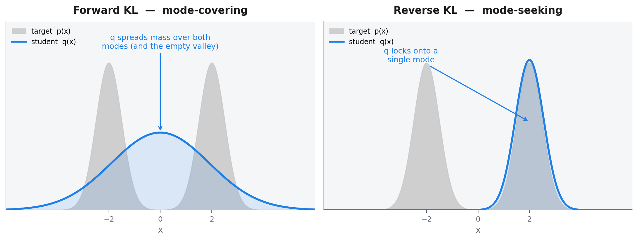
For reasoning and coding, mode-seeking is precisely correct: there is a right answer, and you want the student to converge on producing it, not to hedge across every plausible-looking variant. On-policy distillation uses reverse KL on purpose. One caveat to hold onto, because it comes back later: this is safe only when the student sharpens onto a mode it already shares with the teacher. If the teacher pushes it toward a mode it cannot reach, the same sharpening flips into collapse — which is exactly the stability condition we derive near the end of this part. (Thinking Machines Lab also makes the practical point that this objective is hard to "game": a low reverse KL corresponds directly to high probability under the teacher, so unlike a learned reward model there is no separate scoring network with exploitable blind spots.)

Why dense beats sparse: the efficiency is structural, not incidental

Now the second half of the intuition. Why is per-token feedback such a big deal compared to RL's one-reward-per-attempt?

The intuition. Imagine grading an essay two ways. Way one: you read the whole thing and write a single number at the top, 71/100. Way two: you mark every sentence, this one is sharp, this one buried the point, this transition doesn't follow. The second student learns far faster, because they know which sentences to fix. RLVR is the single number at the top. On-policy distillation is the per-sentence markup.

The mechanism, and where sparse RL actively stalls. RLVR gives one scalar reward per rollout, no matter how many hundreds of tokens the rollout took. Modern RLVR mostly runs on GRPO (group-relative policy optimization). Introduced by DeepSeek in DeepSeekMath (arXiv 2402.03300) and scaled up in DeepSeek-V2, it is the critic-free algorithm nearly every lab in this post builds on. GRPO turns that one scalar into a learning signal by comparing rollouts within a group: it takes several attempts at the same prompt and normalizes their rewards into an advantage, using the group's own average as the baseline instead of a separate learned value network.

Read what happens when a problem is either too easy or too hard: every attempt in the group earns the same reward, all correct, or all wrong. Then each reward equals the group average, so the numerator r_i − mean(r) is zero for every rollout, and every advantage is zero. There is no gradient at all; the group teaches nothing. On hard problems where the verifier almost never fires, that all-wrong case is not a rare edge: it is the common one, which is why RLVR can grind for thousands of GPU-hours making little headway on the hardest material. A dense per-token signal has no equivalent dead zone: even a "failed" trajectory still carries a learning signal at every position. (The standard-deviation denominator is itself contested. It rescales each group by its own spread, so tiny reward differences in a nearly-tied group get blown up while a widely-spread group's get shrunk, arguably muting exactly the rollouts that most deserve a push; several recent GRPO variants drop the std term for this reason.)

The evidence. The measured gaps are large:

• Sample efficiency (MOPD). In the MOPD paper's experiments, on-policy distillation reaches the teacher-level plateau "on IF within ∼25K IF samples and on SWE within ∼30K SWE samples, whereas Mix-RL requires the full 150–180K sample budget in each domain": roughly a 6× reduction in samples to reach the same quality.
• Wall-clock cost (Thinking Machines Lab). On a math-reasoning benchmark, on-policy distillation reached 74.4% in about 1,800 GPU-hours, versus RL's 67.6% in about 17,920 GPU-hours (roughly one-tenth the compute) with off-policy SFT trailing at 60% even after 400K samples.
• Self-distillation (Thinking Machines Lab). Distilling an RL-trained model back into its own base recovered teacher performance with 7–10× fewer gradient steps and 50–100× less compute.

You will sometimes see this compressed to a slogan like "3–10× cheaper." Resist quoting a single number: there is no one figure in any paper that says it. The honest synthesis is roughly 5–10× more efficient than RL, depending on the domain and exactly what you measure, and the reason is the one structural fact above. One scalar per rollout versus a gradient on every token.

The deep layer: three ways to compute the loss, and the one law that governs stability

Everything so far a newcomer can stop at and still have the picture: student solves, teacher grades every token with mode-seeking reverse KL, and that is dense-and-on-policy, which is why it is efficient and parallelizable. What follows is the practitioner's layer, the exact math the labs argue over, and it comes down to two questions: how do you compute that per-token KL, and which teacher is safe to use.

The three loss forms

The reverse-KL objective above is exact but expensive to compute directly, because "the teacher's full next-token distribution" means a probability for every one of the model's 100k+ vocabulary tokens at every position. The MOPD paper lays out three ways to handle it, in increasing cost and stability.

1. Policy-gradient form (the light one; MOPD's default). Instead of computing the full distributional KL, optimize the reverse KL with the REINFORCE trick over a single sampled token. The loss is the policy-gradient objective, each token weighted by an advantage:

The per-token advantage Â_t is just the log-probability gap between teacher and student on the token the student actually produced:

The sg[·] is a stop-gradient, and the advantage is clipped to a fixed range (A_max = 5 in the MOPD paper) so a single wildly-improbable token cannot blow up the update. This form is in the lineage of MiniLLM (Gu et al., ICLR 2024), which first framed reverse-KL distillation as a policy-gradient problem. Its great virtue is what the teacher has to provide: only the log-probability of one already-chosen token. That makes the teacher maximally cheap to serve.

2. Top-k form (k = 64). Instead of one sampled token, match the student to the teacher across the teacher's k most likely tokens at each position (MOPD uses k = 64), with a correction constant so the objective is still minimized exactly at π_θ = π_teacher:

The sum runs only over T_k, the teacher's top-k tokens, so each position moves 64 probabilities rather than one sample or the full 100k-way distribution. The correction C_k, in the paper's words, "ensures the loss is minimised at π_θ = π_teacher on the top-k tokens" — without it, truncating to the top-k would move the minimum and bias the student. This is a richer signal per step than the policy-gradient form and far cheaper than the full distribution, but it asks the teacher to expose its top-k probabilities (more than the single log-prob the first form needs), and, as we are about to see, it is the most fragile of the three when teacher and student disagree.

3. Full-vocabulary form. Compute the exact reverse KL over the entire vocabulary V at every position — the objective exactly as first written, with nothing sampled or truncated away:

Now the inner sum runs over all of V (100k+ tokens), so every position is matched against the teacher's complete next-token distribution. This is the most faithful and the most stable of the three — no sampling noise, no truncation to move the minimum — but it means the teacher must emit, and you must move and store, a full 100k-way distribution at every single position. That is the serious engineering problem at scale, and Part 2 shows the trick DeepSeek uses (caching each teacher's hidden states and rebuilding the logits on the fly) to make full-vocabulary distillation affordable.

Which to pick? MOPD's ablation is reassuring for anyone who wants the cheap option: with a well-matched teacher, the policy-gradient and top-k forms land in essentially the same place, at normalized scores of 0.937 (policy-gradient) and 0.909 (top-k). So the heavier top-k machinery buys almost nothing when teacher and student are close. And when they are not, it is actively worse: in the paper's mismatched-teacher runs the top-k form diverges, while the lighter policy-gradient form only degrades. That "with a well-matched teacher" caveat is doing enormous work, and it brings us to the one result in this whole area you cannot afford to get wrong.

The stability law: a stronger teacher can make things worse

The intuition. You would assume that if you are going to have an expert grade the student, a better expert is always better. For on-policy distillation, that assumption is false, and understanding why is understanding the whole method.

The mechanism. Recall that the student learns from reverse KL over its own samples. The gradient at each token is weighted by the log-probability gap between teacher and student. Now suppose the teacher is much stronger and different: it solves problems in ways the student would never attempt. Then the student's own rollouts routinely land in regions the teacher considers very improbable. In those regions the reverse-KL term log π_T − log π_θ goes sharply negative, a large punitive gradient, because log π_T heads toward negative infinity as the teacher's probability heads toward zero. The student's only escape is to stop producing anything the distant teacher dislikes, which means collapsing its own diversity: entropy contracts, exploration dies, and the model narrows onto a single mode. The signal meant to teach it instead crushes it.

The evidence (MOPD). The MOPD paper demonstrates this cleanly. They swap the well-matched teacher for a stronger external one (Qwen3-235B-A22B). The student's initial per-token KL to the teacher jumps from about 0.04 to about 0.19, roughly 5× more distant at the start. Under the policy-gradient form the student's entropy contracts from 0.30 to 0.21 as it "narrows toward a single mode," driven by the "punitive gradient signal from the teacher's low-probability region," and accuracy degrades. Under the more aggressive top-k form it is worse: training "diverges catastrophically around step 18."

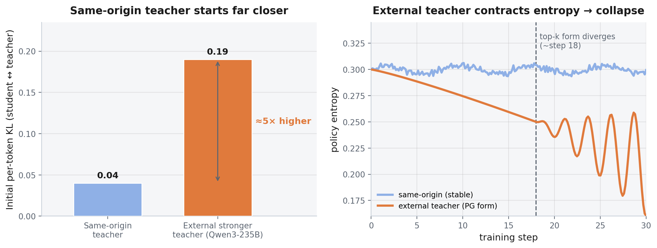
The rule this establishes. The teacher and student have to stay distributionally close, which in practice means a low initial KL between them. A stronger teacher that is also distant does not lift the student; it collapses it. The two main sources frame that requirement from different angles, and it is worth seeing both. The MOPD paper treats same-origin teachers as the critical ingredient: branching every specialist teacher and the student from the same SFT checkpoint is what ensures the low initial KL, and the paper's finding is that this closeness is genuinely required, not an optional nicety you can skip when the distributions feel close enough. Thinking Machines Lab comes at it from the opposite side: it shows that even a size-mismatched teacher and student can distill successfully, so long as their distributions stay close. Read together, the two are compatible, and they point to the same underlying variable. Closeness is the real requirement; branching from a shared checkpoint is simply the most reliable way to guarantee it, and a shared origin is not magic in itself. That through-line is why the technique fuses same-scale specialists that share an origin, rather than trying to compress a giant foreign teacher into a small student. Those are different problems, and Part 2 shows a lab, Alibaba's Qwen3, doing the second one under the same word, "distillation," to very different ends.

The same rule, one layer down. Both instabilities share one root: learning wobbles whenever the distribution you train on drifts from the distribution you actually sampled from. "Keep the distributions close" is really that single principle, showing up at two layers. One layer is the teacher, where a distant teacher pushes the student toward tokens it would never have produced. The other is the plumbing: the model that generates rollouts (a fast inference server) and the model that trains on them run the same weights in slightly different numerical setups, so each update is computed against tokens sampled from a subtly different distribution. Same pathology, one layer down, and at scale it is enough to make training collapse. The labs that productionized this recipe fix it the same way, by filtering the mismatched tokens out. Ant's Ring-1T introduced IcePop, which computes each token's train-versus-inference probability ratio and masks or clips the ones that are badly off in either direction, so the most mismatched tokens never reach the gradient; Zhipu's GLM-5 and Xiaomi's MiMo both adopt it (GLM-5 drops its KL-regularization term). Meituan's LongCat uses a related but distinct truncated-importance-sampling scheme. The lesson generalizes: whenever the thing you learn from drifts from the thing you actually sampled, learning destabilizes, so you keep them close, whether "them" is teacher-and-student or generate-and-train.

The one rule you can't break: keep the teacher and student close. A distant teacher collapses the student instead of lifting it.

It really is "one line changed on an RL script"

The reason labs adopted this so fast is that, mechanically, it is a tiny change to infrastructure they already run. MOPD makes the point directly: it "cast[s] MOPD distillation as an RL process" that "drops directly into existing PPO/GRPO" pipelines, where "the advantage computation is the only change." In pseudocode, a normal GRPO loop versus its on-policy-distillation variant differ by one line:

# Standard RLVR / GRPO inner loop
for prompt in batch:
    responses = student.sample(prompt, k=G)          # student rolls out, on-policy
    rewards   = [verify(r) for r in responses]        # ONE scalar per rollout (sparse)
    adv       = (rewards - rewards.mean()) / rewards.std()   # group-relative advantage
    loss      = -(adv * logprob(student, responses)).mean()
    loss.backward()

# On-policy distillation: same loop, advantage swapped for a per-token teacher gap
for prompt in batch:
    responses = student.sample(prompt, k=G)          # unchanged: student rolls out, on-policy
    with torch.no_grad():
        adv = teacher.logprob(responses) - student.logprob(responses)  # DENSE, per token
        adv = adv.clamp(-A_MAX, A_MAX)               # A_MAX = 5
    loss = -(adv * logprob(student, responses)).mean()
    loss.backward()

The rollout engine, the optimizer, the distributed setup: all unchanged. You replace a sparse scalar reward with a dense per-token gap to a teacher. That is the entire code delta, and it is a big part of why a technique that was already reaching production in mid-2025 and was cleanly written up that October spread so quickly across much of the open frontier.

The payoff: capabilities as microservices

Now pull the threads together, because the reason this matters is bigger than an efficiency win.

On-policy distillation is the one integration method that is dense, on-policy, and parallelizable at once. Look hard at that last word. Because integration is now a cheap, stable, final step (a student sampling while same-origin teachers grade its tokens) the production of capabilities and their integration have come apart. You can build your math specialist, your code specialist, and your instruction-following specialist as independent RLVR jobs, each with its own data, its own verifier, its own schedule, run by different teams that never block one another, and then fuse them, at the end, with a distillation pass that costs a fraction of any one of them.

That is the real reason a growing number of labs are moving this way, and it amounts to a principle: capabilities are becoming microservices. Produce them independently and in parallel; integrate them cheaply at the interface. The old monolith, one enormous multi-domain RL run where every capability is entangled with every other, and touching one means rebuilding all of them, is giving way to something that looks more like a well-factored engineering organization. RLVR does not disappear when a lab works this way; it changes jobs. It stopped being the thing that integrates abilities and became the thing that produces the specialists. Integration is now on-policy distillation's job — whether that means fusing separately-built specialists into one model or having a model distill from its own earlier stages to recover what later training eroded. Part 2 shows both.

If you take one idea from Part 1, take that one. It is the lens that makes sense of every lab's recipe, and of the compute bill behind them.

Part 2 puts the lens to work: how DeepSeek, Xiaomi, Zhipu, Kwai, and Meituan each actually build their models (they differ in instructive ways, down to the exact loss forms), how the same recipe is converging across other labs like NVIDIA, and what this three-engine workload means for the GPUs you provision.

References (Part 1)

• Thinking Machines Lab, On-Policy Distillation (Kevin Lu et al., 27 Oct 2025) — https://thinkingmachines.ai/blog/on-policy-distillation/
• MOPD: Multi-Teacher On-Policy Distillation for Capability Integration in LLM Post-Training (Xiaomi LLM Core) — arXiv 2606.30406
• Tülu 3: Pushing Frontiers in Open Language Model Post-Training (Allen Institute for AI) — arXiv 2411.15124
• DeepSeekMath (DeepSeek-AI) — arXiv 2402.03300
• MiniLLM: Knowledge Distillation of Large Language Models (Gu et al., ICLR 2024)