Building a Point-in-Time Finance LLM on 8×H100 + Qwen3.5-35B: A Full-Weight Recipe

TL;DR
What this is: If a trading firm wants a finance LLM with lookahead bias under control, the smallest practical entry point is 8×H100 and a 35B base model. This post records how we set that unit up. We ran continued pretraining onQwen/Qwen3.5-35B-A3B-Baseover 1 billion point-in-time tokens, then measured whether the leakage premium shrank using R². It covers (1) how we measure the leakage and what we found, (2) a control experiment separating whether the leakage is pretraining-driven, and (3) a comparison against the same measurement run with single-GPU LoRA — and then, in an appendix, (4) why a single H100 can't do this and the four troubleshooting passes it took to fit full-weight 35B onto 8×H100. This experiment is inspired by Bryan Kelly and collaborators' research on point-in-time language models, applied here to a commercial-grade 35B base.
Korean blog post
Companion cookbook: multi-GPU cookbook.
The problem a finance prediction LLM has to clear

Robinhood recently opened an "agentic trading" platform for its clients, letting anyone hand investment decisions to an AI agent — a sign of how quickly AI-driven trading is going mainstream. At the top end, the spend is enormous: Jump Trading said at GTC Taipei it would be among the first to deploy NVIDIA's next-generation Vera Rubin (NVL144) platform, while Jane Street committed $6 billion to CoreWeave for AI-cloud capacity.
As agentic trading becomes the norm, a trading firm can only secure alpha by tuning its own model's performance to its own proprietary strategy. But taking a commercial open-source LLM straight off the shelf runs into one large problem: when its data was trained.
Open-source LLMs are mostly trained on data scraped from across the internet. If the training cutoff is 2024, every document published up to 2024 is baked into the model.
So when you ask the model to "predict 2018 returns as of 2017," a problem shows up. On the surface it looks like a 2017-vintage prediction, but the model may have already seen 2018 news articles or reports during training. This is what the academic literature calls lookahead bias: clues that were not knowable at the past point in time stay inside the model and can shape the prediction.
For a trading firm, that undermines backtest credibility. It becomes hard to tell whether a result is "real alpha" or "an artifact of the model having seen the future."
On the academic side, Bryan Kelly (Yale SOM, AQR) and collaborators addressed this with point-in-time language models (Kelly et al., "Scaling Point-in-Time Language Models"). They cut the data chronologically so a model only sees text published up to each point in time, and trained decoders up to 4B parameters. This structurally reduces the problem of future documents bleeding into the training set. A 4B model is enough to validate the principle, but a trading firm weighing 30B–70B class bases needs a recipe at a larger scale.
This post has a different goal: a recipe that applies the same point-in-time principle to a commercial-grade 35B base, plus the measurement tooling to check whether the result is statistically meaningful.
The measurement tool: the gap between two R² values
The core idea is to score one trained model two ways — not to build two training sets. We take the same model, measure it on the Kaggle JPX (a Japan Exchange stock-prediction Kaggle competition) data under two evaluation protocols; looking at the gap is the goal.
- R² leakage-off (chronological split): a time-respecting evaluation. Train on everything before 2020-12-31 and test on everything after 2021-01-01, so no future information leaks into the evaluation. This score is close to true as-of-the-past prediction performance.
- R² leakage-on (GroupKFold on SecuritiesCode): split train and test by stock only. The same stock never lands on both sides, but the dates can mix. So the time leakage of other stocks' future dates entering the training fold remains.
- leakage premium = r2_on − r2_off: how much the time leakage inflated the score.
We compare two models. One is the untrained Qwen/Qwen3.5-35B-A3B-Base; the other is the same base with 1 billion point-in-time tokens of continued pretraining. We compute each model's leakage premium, then take the base premium minus the continued-pretraining premium (premium_reduction) to see how much the use of leakage shrank.
The research hypothesis is this: continued pretraining on 1 billion point-in-time tokens pushes premium_reduction meaningfully above zero.
We check statistical significance with a clustered bootstrap. We resample 200 times at the stock level across 1,000 stocks and watch how much the result moves. If the resulting 95% confidence interval (CI) includes zero, that means "we cannot conclude a reduction."
The shape of the recipe
Here are the fixed values of the recipe we ran on 8×H100.
| Item | Value |
|---|---|
| Base model | Qwen/Qwen3.5-35B-A3B-Base (35B total, about 3B active per token in an MoE structure) |
| Data | HuggingFaceFW/fineweb, CC-MAIN ≤ 2017-W26 (week 4 of June 2017) dump slice |
| Token budget | 1B tokens |
| Training method | Full-weight continued pretraining (training all 35B parameters of the base) |
| Distributed training | axolotl 0.16 + FSDP2 + activation checkpointing off |
| Optimizer | adamw_torch_fused (PyTorch's default AdamW, the fused version that runs fast on the GPU) |
| Precision | bf16 |
| GPU | 8×H100 SXM (one server tied together with NVLink) |
| Training time | 18 hours 36 minutes (train_runtime, measured) |
| Training cost | about $378 (8×H100 node wall-clock ~19.8 hours × $19.12/hour, billed; train_runtime is 18h36m) |
| Evaluation | Kaggle JPX, 1,000 stocks × 30 evaluation dates, 200 bootstrap draws |
MoE (Mixture of Experts) packs 256 small expert networks into one model. Each token activates only a few of them. The full model is 35B, but processing a single token activates about 3B parameters.
With this config, the real run finished 56,430 steps and epoch 1.0 in 18 hours 36 minutes by train_runtime (final train loss 2.182). The merged weights are stored in VESSL Cloud's Object storage (merging those weights after training ended had a story of its own, which we wrote up in Appendix B). How we arrived at this config, and why a single H100 can't finish this training, are in the appendix at the end. First, let's look at what the training measured.
Measurement results
The evaluation reused the exact tooling from the LoRA cookbook: 1,000 stocks × 30 evaluation dates, a test sample of about 5,817, time order preserved, 200 bootstrap draws. Training took 18 hours 36 minutes by train_runtime (job wall-clock about 19.8 hours); evaluation took about 2 hours 50 minutes. The training job billed about $378; adding the offline merge and evaluation brings the total to about $386.
| Metric | Base (untrained base) | Full-weight (this run) |
|---|---|---|
| r2_leakage_off (future-blocked evaluation, chronological split) | −0.1936 | −0.1577 |
| r2_leakage_on (future-leaking evaluation, GroupKFold) | −0.0562 | −0.0678 |
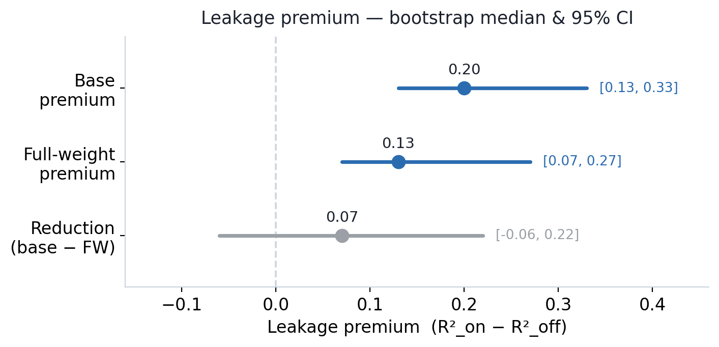
| leakage_premium = median [95% CI] | 0.20 [0.13, 0.33] | 0.13 [0.07, 0.27] |
| premium_reduction (base minus this run) = median [95% CI] | (baseline) | 0.07 [−0.06, 0.22] |
Reading it is simple. If the CI excludes zero, the reduction is statistically meaningful. If the CI includes zero, it means "the direction is right but not significant." In that case you need to tighten the confidence interval. Raising the stock count or the token budget is one route, but as the ChronoGPT section below shows, the evaluation protocol itself may be a more direct lever.
For a trading firm, all three outcomes carry meaning.
- If the full-weight CI excludes zero: that is data showing 1B-token point-in-time full-weight continued pretraining reduced the leakage premium by a statistically meaningful margin. It becomes evidence that 8×H100 + a 35B base produces a measurable capacity to shrink that premium.
- If the full-weight CI includes zero: it means today's setup (1B tokens / 1,000 stocks) alone can't catch a significant reduction. The next experiment's direction is to tighten the CI — and the candidates include not just the token budget or evaluation stocks but the evaluation protocol (see the ChronoGPT section below).
- If R² itself stays negative: point-in-time continued pretraining did not produce absolute alpha (excess return above the market average). What this tool looks at is the reduction in leakage premium, not the discovery of new alpha.
We also checked whether this premium is pretraining lookahead
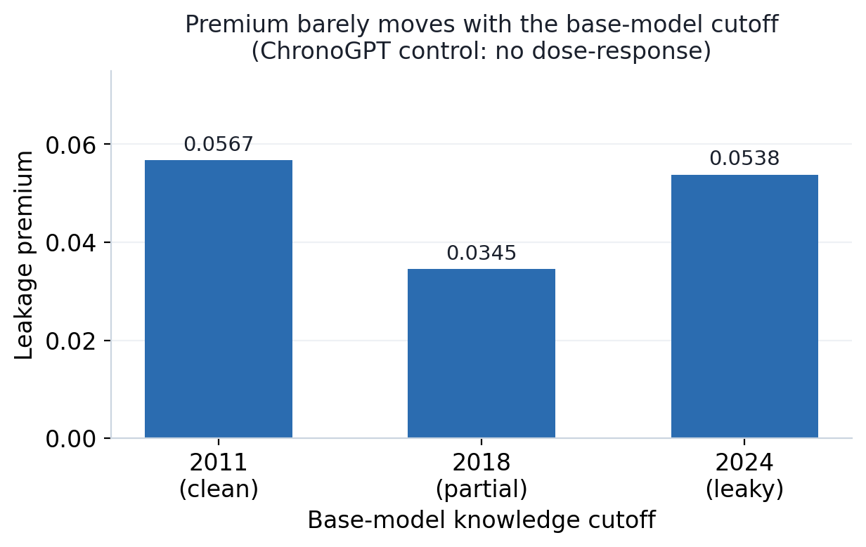
One thing is worth pinning down. Is the leakage premium measured above really there because "the model saw the future during pretraining," or is it an effect of the evaluation protocol, where GroupKFold mixes dates? The two mean different things. If it is the former, moving the base model's knowledge cutoff later should grow the premium. If it is the latter, the premium stays about the same regardless of the cutoff.
The way to separate them is to swap the model by knowledge cutoff. We dropped ChronoGPT (a point-in-time model series released by ManelaLab, trained to see text only up to 2011, 2018, and 2024; the He et al. 2502.21206 paper in Related below is from the same group) into the base slot, kept the evaluation tooling and the JPX data fixed, and re-measured the premium.
| Model knowledge cutoff | JPX evaluation window (after 2021) | leakage premium |
|---|---|---|
| 2011 | never saw it (clean) | 0.0567 |
| 2018 | partial | 0.0345 |
| 2024 | saw it (leaky) | 0.0538 |
The result pointed one way — though the control itself has weak statistical power. Moving the knowledge cutoff from 2011 → 2018 → 2024 did not grow the premium monotonically (0.0567 → 0.0345 → 0.0538; the 2024 model that saw all of it was actually lower than the 2011 model). The difference between the 2011 model that never saw anything after 2021 (premium 0.0567) and the 2024 model that saw all of it (premium 0.0538) is just −0.003, with a 95% confidence interval from −0.40 to 0.07 that runs well across zero (1,000 stocks, 200 bootstrap draws). In other words, there is no dose-response signal from moving the cutoff. The CI is wide enough that we can't claim "no effect at all," but at minimum we found no evidence that the premium moves with the pretraining cutoff.
So the premium we measured in this post is not the "model saw the future during pretraining" kind of lookahead. It is the evaluation-protocol time leakage that comes from GroupKFold mixing dates, the same leakage defined in the measurement-tool section above. Lookahead bias as a concept still stands as a reason to weigh point-in-time training. But at least in this control experiment, the number points to the evaluation design rather than the model's pretraining memory. In the same vein, premium_reduction reads more accurately as "35B continued pretraining had almost no effect on the leakage produced by the evaluation protocol" than as "we erased pretraining leakage."
We also stress-tested the baseline: an embargoed split and a walk-forward
The premium so far rests on one chronological split (train ≤ 2020-12-31, test ≥ 2021-01-01). Two cheap robustness checks, run on the same base and full-weight checkpoint, ask whether that one split is hiding anything.
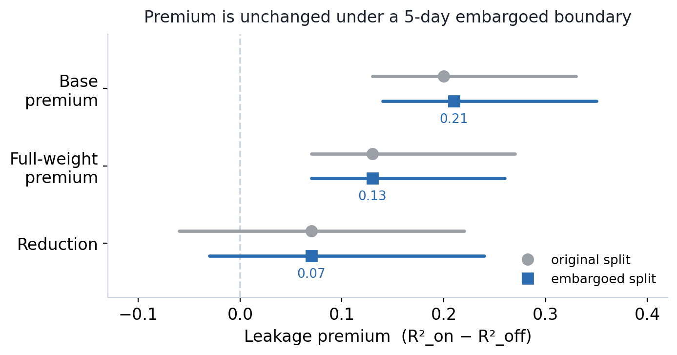
An embargoed boundary. JPX's target is a forward return about two trading days out, so a split that trains right up to 2020-12-31 could let the label horizon straddle the boundary — a thin slice of lookahead the split never intended. We re-scored the chronological r2_leakage_off with a 5-day embargo: same post-2021 test window, but drop the trading days immediately before the cut. The honest score barely moves — base −0.19 → −0.20, full-weight stays −0.16 — so the chronological baseline wasn't leaking at its edge. The premium is essentially unchanged from the headline: base 0.21 [0.14, 0.35], full-weight 0.13 [0.07, 0.26] (both CIs still exclude zero), reduction 0.07 [−0.03, 0.24] (median [95% CI]). So the premium is not an artifact of an un-purged split edge, and the reduction stays non-significant. One scope note: this purges the boundary of the honest split; it does not replace the date-mixing GroupKFold on the leaky side with a purged time-series CV. That larger eval-protocol rework is still the open lever flagged above.
A walk-forward. An expanding walk-forward (five folds, pooled R²) scores more than one test window: base −0.25, full-weight −0.27, both more negative than the single 2021 split. The no-alpha read holds across periods, not just at one boundary. (The full-weight run is fractionally worse here than on the 2021 split; its small edge over the base there doesn't carry across periods — one more reason to read this as 'no alpha,' not 'the training helps.')
How this differs from Bryan Kelly's team
Bryan Kelly's group at Yale — also affiliated with AQR Capital Management — trained a 4B-parameter model from scratch on point-in-time-filtered text, structurally shutting out any inflow of future information at the source.
We started from the opposite end: a commercial 35B base that had already absorbed the entire internet through 2024, onto which we ran 1 billion tokens of continued pretraining (CPT). The two experiments begin from fundamentally different starting points.
We ran the same measurement with single-GPU LoRA too
In the Single-H100 LoRA cookbook we're publishing alongside this post, we ran a variant that trains only a LoRA (Low-Rank Adaptation — a small adapter that leaves the model body intact and trains only small adapter matrices) adapter on the same base (Qwen/Qwen3.5-35B-A3B-Base) and the same 1B-token FineWeb slice. That is about 945M parameters, roughly 2.6% of the full model. It went through the same evaluation tooling.
Here is the difference.
| Metric | LoRA variant | Full-weight variant (this post) |
|---|---|---|
| Trained parameters | about 945M (about 2.6% of the whole) | 35B (all) |
| Training time | 23 hours 23 minutes (1×H100 SXM) | 18 hours 36 minutes (8×H100 SXM) |
| Training cost | about $56 | about $378 |
| premium_reduction (median [95% CI]) | 0.065 [−0.05, 0.18] | 0.07 [−0.06, 0.22] |
| Does the CI exclude zero? | No (directional but not significant) | No (directional but not significant) |
The LoRA variant's premium-reduction CI included zero. So this full-weight run had a clear job: separate whether the problem was the 97% of parameters LoRA never touches, or the 1B-token, 1,000-stock setup itself.
The answer is closer to the latter. The full-weight run's reduction CI also included zero. So the 97% of parameters LoRA froze was not the key bottleneck. And as the ChronoGPT section just above showed, the premium itself comes largely from the evaluation protocol, so raising the token budget alone may not be enough to push this CI off zero.
On cost, full-weight is about 6.8× LoRA. But it did not buy a tighter CI. Both variants' reduction CIs included zero. Still, the base leakage and the post-training residual leakage both excluded zero in both. The signal that the measurement tool works consistently held up.
One caveat worth flagging. The LoRA reduction in the table above (0.065) is the published LoRA adapter re-evaluated on this post's own inference stack (transformers 5.2 / torch 2.5); measured the same way, LoRA's 0.065 and full-weight's 0.07 are effectively identical. The Single-H100 LoRA cookbook, by contrast, reports a reduction of 0.11 and a base premium of 0.32 (median) on its own stack (transformers 5.5 / torch 2.10), which can look different from this post's 0.065 and 0.20. But this gap isn't from re-sampling stocks on each eval run. Both evaluations used the same base on the same eval set (a test sample of 5,817 across 1,000 stocks) and the same input data (the raw JPX, 2,332,293 rows). Stock selection is also seed-fixed and deterministic — run the same setup three times and base R² reproduces to four decimal places. The real cause is that the two evaluations embedded the frozen base under different inference stacks. Even on the same base, a different library version shifts the embedding values slightly, and base R² moves with it. So rather than lining up absolute base values across cookbooks, compare the conclusion each evaluation reaches: in both, the base leakage (premium) sits significantly above zero, and one training pass doesn't significantly reduce it (the two base CIs, [0.13, 0.33] and [0.22, 0.53], also overlap).
The detailed LoRA variant recipe (Unsloth single-process, 12 hybrid attention LoRA target locations, the dump-week slice data-prep script, GroupKFold evaluation) is in the Single-H100 LoRA cookbook. This post's companion, the multi-GPU cookbook, covers only the full-weight path.
What a trading firm should take away
- The measurement tool worked. One run did not produce a meaningful reduction. We re-measured the principle behind Kelly et al.'s separate 4B training on top of a commercial-grade 35B base. The base leakage and the post-training residual leakage consistently excluded zero in both LoRA and full-weight. But the 95% CI on premium reduction included zero in both variants. With today's 1B-token, 1,000-stock setup alone, you can't say "leakage shrank meaningfully."
- Full-weight was used to separate hypotheses. But the real lever may not be the token budget. LoRA alone couldn't separate "is the token budget short, or are the 97% of untrained parameters the drag?" So we ran 8×H100 + 35B full-weight once. The result is clear: the 97% of parameters LoRA froze is not the key bottleneck. But as the ChronoGPT control test above shows, the premium is nearly independent of the model's knowledge cutoff — it looks largely like an evaluation-protocol effect. If so, raising the token budget alone may not push the reduction CI off zero. The more direct lever is likely the evaluation protocol itself (for example, a purged time-series cross-validation that does not mix dates).
The four troubleshooting passes and the config differences are recorded in the appendix below and, experiment by experiment, in the companion multi-GPU cookbook.
Run it on your own portfolio data
If you're weighing the same point-in-time full-weight continued pretraining on a 30B–70B base, or you want to measure leakage premium directly, VESSL Cloud's 8×H100 SXM tier is the entry point. The companion cookbook above is a recipe you can follow start to finish. For a 70B+ base or multi-node training, reach out at sales@vessl.ai — VESSL Cloud runs a full GPU range, from L40S to B300.
Run this setup yourself, talk to the VESSL Cloud team →
Below is the engineering record of getting the recipe above actually running on 8×H100. If you don't care about FSDP2 memory debugging, you can stop here.
FAQ
Did this produce alpha or a profitable model?
No. Both out-of-sample R² values are negative. What this measures is the leakage premium — how much a date-mixing evaluation inflates the score — not new alpha.
Why train full-weight instead of just a LoRA?
To separate two explanations for why one pass didn't significantly cut the premium: the ~97% of parameters a LoRA never touches, or the 1B-token / 1,000-stock setup itself. The full-weight reduction CI still crossed zero, so the frozen parameters weren't the bottleneck.
Is the leakage premium real, or a statistical artifact?
Real and significant — the base and post-training premium CIs both exclude zero. But the ChronoGPT control shows it comes mostly from the evaluation protocol (GroupKFold mixing dates), not from the model seeing the future during pretraining.
Can I run this on fewer than 8 GPUs?
Full-weight 35B needs 8×H100 — a single 80 GB H100 can't hold the ~420 GB of optimizer state, so FSDP sharding across 8 cards is required. The single-H100 LoRA variant runs on one card (about $56). For a GPU-by-GPU cost picture, see our A100 vs H100 vs B200 cost benchmark.
Where's the runnable code?
Both recipes are open on GitHub — the single-H100 LoRA cookbook and the 8×H100 full-weight cookbook.
Appendix A — Why a single H100 can't finish it
The reason is simple: memory.
Training all of 35B starts with looking at what gets loaded onto the GPU. Storing 35B parameters in bf16 makes the model itself 70 GB. That barely fits on a single 80 GB H100.
But training needs more than the model. The AdamW optimizer carries three extra pieces of information per parameter:
- fp32 master copy: a precise 32-bit copy (4 bytes per parameter)
- m (first moment): an exponential moving average of the gradient (4 bytes)
- v (second moment): an exponential moving average of the squared gradient (4 bytes)
The bf16 model parameters update against the fp32 master copy during training. m and v correct the direction and scale of each update. All three have to sit in GPU memory throughout training.
The arithmetic:
- 35 billion parameters × 4 bytes × 3 = about 420 GB
A single H100 (80 GB) falls short by more than five times. Add activations (the intermediate values computed during the forward pass) and gradients (the update-direction signal computed during the backward pass) and it grows further.
You could force it in with quantization (compressing numbers into fewer bits). But in this experiment, precision can change the result. We avoided any choice that could shake the quality of the measurement.
So a single GPU can't finish it. When a model doesn't fit on one card, you split it across several.
The method for that is FSDP (Fully Sharded Data Parallel). It splits the model parameters, gradients, and optimizer state across N GPUs, 1/N each. During computation, each GPU gathers only the parameters it needs for its turn, then re-splits once the computation is done.
Splitting across 8 GPUs cuts the load sharply. The 420 GB of optimizer state becomes about 52 GB per card; the 70 GB of model weights and 70 GB of gradients become about 8.75 GB each per card. A naive sum is about 70 GB per card — just barely fitting on a single 80 GB H100. That is an upper-bound estimate, though, so the debugging section below confirms with measured numbers how far the actual training pushes memory.
That makes VESSL Cloud's 8×H100 SXM tier the realistic entry point for full-weight 35B training. For bigger jobs such as 70B+ bases or multi-node training, you can also weigh a B200 or Rubin (NVIDIA's next-generation data-center GPU) expansion. If you need the GPUs, reach out at sales@vessl.ai.
Appendix B — Getting it onto 8×H100: four troubleshooting passes
"Possible in theory" and "training actually runs" are different things. The very first experiment hit an OOM (Out of Memory). This section is that debugging log. The measurement results are above, so read on only if the engineering interests you.
The way it didn't fit was odd
There was a good signal first. The 2×H100 LoRA dry-run (a small-scale trial run before the real one) passed cleanly. That meant FSDP2 shards this hybrid attention model (a structure that mixes two different attention mechanisms in one model) well.
The question was whether removing LoRA and letting all of 35B train would still fit in GPU memory.
The first experiment's answer was clear: it didn't. But the reason wasn't obvious right away.
Setup: 8×H100 SXM, axolotl 0.16, FSDP2,
       optimizer adamw_torch_fused, seq_len 4096,
       gradient_accumulation_steps 4

Result: OOM at first backward
        GPU 1: 506 MiB free of 79.18 GiB total,
               75.26 GiB held by PyTorch
        Tried to allocate 1024 MiB → allocation failed
The memory arithmetic alone looked strange. Split across 8 cards, the sharded parameters per GPU are about 8.75 GB, and the sharded gradients are about 8.75 GB too. With activation checkpointing on (a trick that trades compute for memory: it skips storing some intermediate values and recomputes them during backward), the extra parameters needed mid-computation run around 1.75 GB. The activations themselves are a few GB at sequence length 4096.
All together I expected about 20–25 GB per GPU. The measured number was 73–75 GB. It was using roughly 50 GB more than expected.
One more thing was confusing. The OOM happened before the first optimizer.step() (the step where the optimizer actually updates parameters). The optimizer's extra state had not even been allocated yet.
We then swapped the optimizer to paged_adamw_8bit (8-bit quantized AdamW) and cut the sequence length from 4096 to 2048. Both changes helped narrow the hypothesis. The 8-bit optimizer had no effect: it allocates its state lazily inside the first step, so it has no bearing at the OOM point. Halving the sequence length saved only about 2 GB. The missing 50 GB was still there.
Two hypotheses, and the OOM timing gave the answer
There were two diagnostic candidates.
Hypothesis A: the extra memory is unsharded optimizer state. The idea is that bitsandbytes (the 8-bit optimizer library) doesn't understand FSDP2's DTensor (distributed tensor — the PyTorch structure that tracks sharded parameters), so it allocates an fp32 master copy for the full 35B model on every GPU.
Hypothesis B: the extra memory is unsharded gradients. The idea is that when gradient_accumulation_steps > 1 (collecting several small batches to get the effect of a larger batch), the gradients FSDP holds inside no_sync() (a mode that briefly turns off cross-GPU synchronization while gradients accumulate) are the problem. The PyTorch FSDP docs state this clearly.
FSDP will accumulate the full model gradients (instead of gradient shards) until the eventual sync.
In other words: while gradients accumulate across several microbatches, FSDP holds the full unsharded gradient on each GPU, not the sharded one.
The fact that the OOM happened at the first backward split the answer.
bitsandbytes allocates its optimizer state lazily inside the first optimizer.step(), not at init. If Hypothesis A were right, the OOM should have hit at the first step. But the real OOM landed before a single step ran, at the first backward. Hypothesis A's timing didn't fit.
Hypothesis B, on the other hand, fit exactly. With gradient_accumulation_steps: 4, Accelerate (Hugging Face's distributed-training helper library) suppresses gradient sync on the first three microbatches (the small accumulation batches) of every step. During that no_sync window, FSDP holds the full 35B gradient on each GPU rather than the sharded one.
That is up to 70 GB of unsharded gradient in bf16. Add the sharded parameters, the extra parameters needed mid-computation, activations, and buffers, and you reach 73–75 GB. The measurement and the arithmetic lined up.
To put it plainly: normally FSDP splits the gradient across GPUs every backward, keeping per-GPU memory at 1/N. But under no_sync(), that behavior pauses. The gradient accumulated during that window stays at full model size on each GPU. The model parameters are sharded, but the gradients alone stay whole on each GPU.
The fix was one line.
- gradient_accumulation_steps: 4
+ gradient_accumulation_steps: 1
We reran it. The first backward passed, and training started.
Why this is confusing. Gradient accumulation is usually a memory-saving tool. You stack small batches to train as if with a large one, so it's the natural option to reach for when you OOM. But FSDP inverts that expectation. Because ofno_sync(), the gradient stays unsharded during accumulation and can sit at full model size on each GPU. The cookbook's final config setsgradient_accumulation_steps=1explicitly, with a comment citing the PyTorch docs.
The final cleanup: optimizer and activation checkpointing
The gradient-accumulation fix was the structural solution, but it wasn't the end. paged_adamw_8bit died right away in optimizer.step() with a RuntimeError.
RuntimeError: mixed torch.Tensor and DTensor
  at bitsandbytes/optim/optimizer.py:520
  → optimizer_update_32bit
This is the incompatibility tracked in bitsandbytes #1633. The 8-bit Adam state-update kernel (a small function that runs on the GPU) didn't know how to handle the sharded parameters wrapped in FSDP2's DTensor.
Next we swapped the optimizer to adamw_torch_fused. PyTorch builds it directly, it's FSDP2-compatible, and there's no DTensor confusion. It has a cost: about 17.5 GB of sharded fp32 master copy per GPU on top of what the 8-bit optimizer would use. But the gradient-accumulation fix had freed 50 GB, so there was room. With activation checkpointing on, peak memory settled at about 42 GB.
Finally, we turned activation checkpointing off. Instead of recomputing intermediate values during backward, we just keep them in memory. That uses more memory but speeds training up. The adamw_torch_fused profile peaked at 42 GB with activation checkpointing on, leaving about 37 GB of headroom. We could trade that headroom for +32% throughput. On an 18-plus-hour run, +32% is the difference between finishing within a day and overshooting the credit budget. With it off, peak settled at 51 GB, leaving about 29 GB of margin.
Across these fixes, the config stabilized. The real run finished 56,430 steps and epoch 1.0 in 18 hours 36 minutes by train_runtime. Final train loss was 2.182.
Training finished, but the job died
The run completed, yet the job ended in state failed. In chronological order, the log reads:
01:07:30— the last step (56,430 / 56,430, epoch 1.0) passed. The training math was done here.01:21:28— the Trainer printedTraining completed!and safely wrote the sharded checkpoint (checkpoint-56430) to disk. train_runtime of 66,980 seconds (18 hours 36 minutes) was logged here.- Right after, axolotl started consolidating the FSDP shards into one set of weights inside the same distributed job (
merge_sharded_fsdp_weights). While rank 0 wrote the 66 GB consolidated file to Object storage (a network volume), the other 7 ranks sat waiting on a single ALLREDUCE. - That consolidation write ran past 30 minutes. At
01:51:28, the NCCL watchdog flagged the collective as a timeout.
[Rank 1] Watchdog caught collective operation timeout:
  WorkNCCL(SeqNum=7122731, OpType=ALLREDUCE, Timeout(ms)=1800000)
  ran for 1800092 milliseconds before timing out.
→ c10::DistBackendError → all ranks terminated → job state failed
In other words, the training didn't fail — the distributed barrier in the final consolidation step timed out after training was completely done. The checkpoint-56430 we actually needed was already sitting safely on disk. The NCCL watchdog timeout had already been raised from the 10-minute default to 30 minutes, and rank 0's 66 GB network write still blew past it.
The fix was to drop the distribution. We spun up a separate single-process job on one GPU and re-merged the shards from checkpoint-56430 offline (16 shards, 66 GB bf16). With no NCCL barrier, there was no timeout. The evaluation in the results above ran on this merged checkpoint.
The lesson. Running the final consolidation of a large FSDP checkpoint inside the distributed job means rank 0's multi-tens-of-GB write to a network volume can outlast the NCCL collective watchdog — and kill a job whose training is 100% done. So the cookbook's final procedure keeps only sharded checkpoints during training (SHARDED_STATE_DICT) and runs the consolidation afterward in a separate single-process job that needs no distribution. That's how the merged weights ended up in VESSL Cloud's Object storage.Related
- Multi-GPU cookbook: the reproducibility recipe for full-weight 35B continued pretraining on 8×H100: this post's companion (fixed config values, the FSDP2 memory-debugging log, cost, operational checks)
- Single-H100 LoRA cookbook: the same measurement with LoRA: comparison reference (945M adapter, single GPU, about $56)
- Kelly, Bryan, et al. "Scaling Point-in-Time Language Models." SSRN Working Paper No. 6681860. <https://ssrn.com/abstract=6681860>.
- He, Songrun, Linying Lv, Asaf Manela, and Jimmy Wu. "Chronologically Consistent Large Language Models." arXiv:2502.21206. <https://arxiv.org/abs/2502.21206>.
- PyTorch FSDP no_sync() docs
- Accelerate gradient synchronization guide
- bitsandbytes #1633: FSDP2 and 8-bit Adam DTensor incompatibility
VESSL AI
Subscribe to our newsletter
Monthly insights on building AI infrastructure, the latest GPU news, and more.