Speculative Decoding: One Equation & Four Levers

Why are GPUs mostly idle during decode?

Autoregressive generation emits one token per forward pass:

Generating $N$ tokens takes $N$ sequential passes. The dependency is the problem, not the arithmetic.

Consider one decode step on a 70B model in bf16. It reads about 140 GB of weights from HBM to produce a single token. On an H100 at 3.35 TB/s, that is roughly 42 ms, about 24 tok/s. The arithmetic in that same pass is around $2P = 1.4 \times 10^{11}$ FLOPs against a 989 TFLOP/s peak. That is 0.14 ms of compute hiding inside 42 ms of memory traffic.

Decode is memory-bound by two to three orders of magnitude. The GPU is mostly waiting.

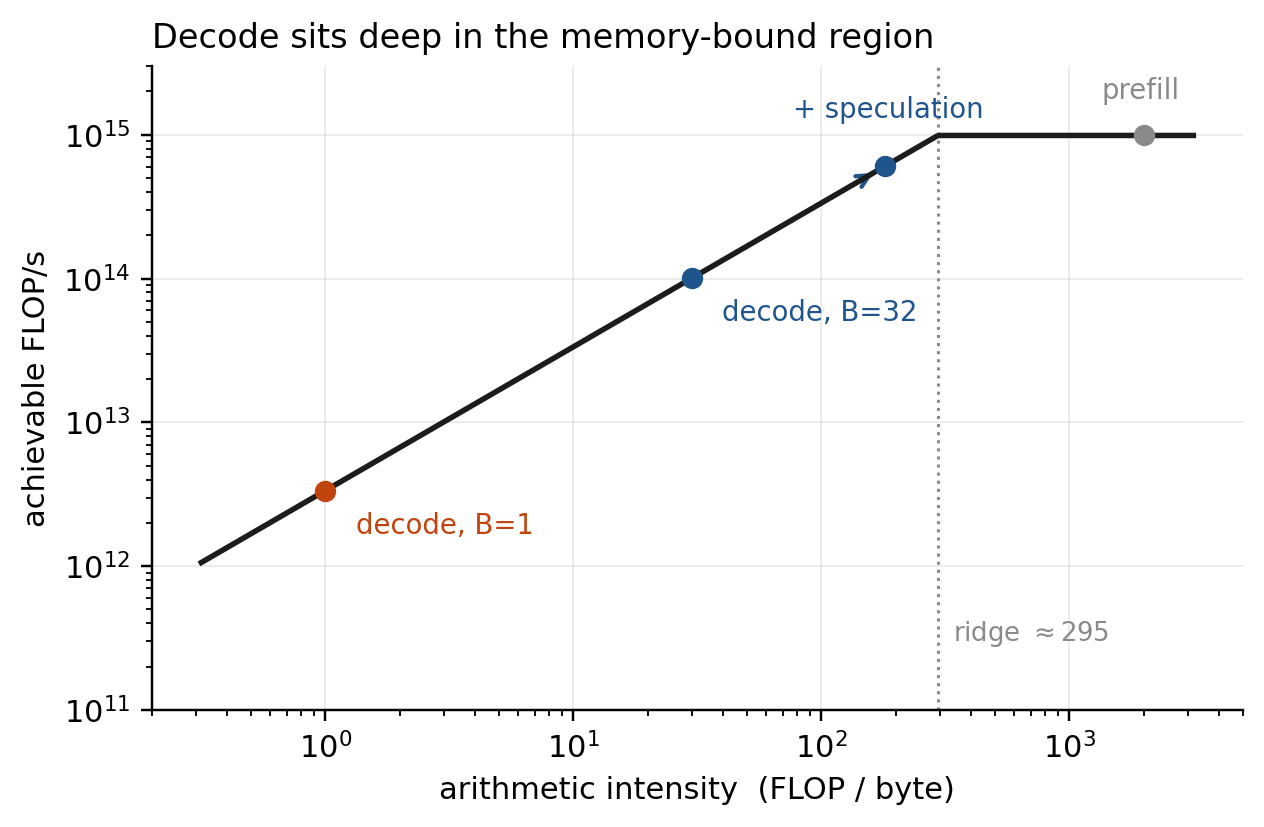
Verifying $\gamma$ drafted tokens in one pass covers $\gamma+1$ positions and multiplies arithmetic intensity by that factor, while leaving weight traffic unchanged. In the flat region that is nearly free. Everything below is a consequence of that flatness.

Most acceleration techniques make each step cheaper. Quantization and sparsity cut bytes per weight. Larger batches amortize weight traffic. Better kernels shave constants. All of them leave the serialization intact.

Speculation is different. It attacks the sequential dependency itself. And it is the only one of these that can be made exactly lossless.

The algorithm for speculative decoding

A cheap drafter proposes $\gamma$ tokens. One target forward pass over $\gamma+1$ positions checks all of them at once. The longest valid prefix commits.

# one speculative cycle
#   prefix x[:i], speculation length gamma
#   M_t = target, M_d = drafter

# --- draft phase: gamma sequential cheap steps ---
for j in range(gamma):
    q[i+j]  = M_d(prefix=x[:i] + draft[:j])
    draft[j] = sample(q[i+j])

# --- verify phase: ONE target pass over gamma+1 positions ---
p[i : i+gamma+1] = M_t(x[:i] + draft, causal_mask=True)

r = uniform(0, 1, size=gamma)
n = first_index_where(r > p[i+j][draft[j]] / q[i+j][draft[j]])   # or gamma

emit(draft[:n])                                   # n accepted tokens
if n < gamma:
    emit(sample(normalize(relu(p[i+n] - q[i+n]))))  # corrected token
else:
    emit(sample(p[i+gamma]))                        # free bonus token

truncate_kv_cache(to=len_emitted)

Two things to notice. The $\gamma$ ratio tests happen in parallel after one target pass, so verification has no sequential dependency, which is the entire point. And a rejection still emits one corrected token, so $\tau \geq 1$: speculation never stalls.

The idea comes from branch prediction in CPUs, but two differences matter in practice. A CPU misprediction is a correctness event; an LLM rejection is a statistical one. A drafted token can be perfectly reasonable text and still get rejected, because the test is distributional identity, not correctness. And a CPU pipeline flush is cheap, whereas LLM rollback is cheap only because the KV cache is append-only, a premise that breaks for recurrent-state and linear-attention layers.

The acceptance rule

Draw $x \sim q$ from the drafter. Accept with probability $\min\!\big(1, \tfrac{p(x)}{q(x)}\big)$. On rejection, sample the replacement from the normalized residual:

The intuition: $q$ gives too much mass to some tokens and too little to others. The ratio test removes the excess. The residual is exactly the deficit, renormalized.

Theorem (losslessness). The emitted token is distributed exactly as $p$.

Proof. Let $\beta = \sum_u \min(p(u), q(u))$. The acceptance path contributes $q(x)\min\!\big(1, \tfrac{p(x)}{q(x)}\big) = \min(p(x), q(x))$. The rejection path contributes $(1-\beta)\,p'(x)$, and since the normalizer equals $1 - \beta$, that is exactly $\max(0, p(x) - q(x))$. Summing:

The proof uses no property of $q$ at all. That single fact opens the whole design space: n-gram tables, suffix automata, diffusion models, quantized networks, the target with half its layers skipped. All legal, all lossless, no change to the correctness argument.

So every improvement to the drafter is purely an efficiency improvement. Inside the lossless branch there is no quality trade-off.

And the acceptance rate has a closed form:

This identity is from Leviathan et al. (2023), where the divergence carries their own name $D_{LK}$ and the per-prefix rate is kept separate from its expectation over prefixes. It turns a systems question (how often does the fast path fire?) into a statistics question: how close are two distributions in $L_1$. That is what makes drafter training a well-posed optimization with a known optimal objective, and it is why the rest of this post can be arithmetic rather than intuition.

Two corollaries people get wrong. Top-1 agreement is not $\alpha$, except at temperature 0. And $\alpha$ is per-position: any single number you have been quoted is an average over an unstated mix of contexts.

What determines the speedup | one equation

Assume acceptance is i.i.d. $\text{Bernoulli}(\alpha)$, and let $c = T_{\text{draft}} / (\gamma \, T_{\text{target}})$ be the drafter's relative cost, where $T_{\text{draft}}$ is the wall time of the whole $\gamma$-token draft phase rather than one drafter step. Expected tokens per cycle is a truncated geometric:

A cycle costs $(c\gamma + 1)\,T_{\text{target}}$. Dividing gives the speedup equation, also from Leviathan et al. (2023):

Three parameters: $\alpha$, $c$, $\gamma$. Almost every speculative decoding paper intervenes on one of four terms:

Lever	What it does	Examples
$\alpha \uparrow$	make the drafter's $q$ closer to the target's $p$, so drafts are accepted more often	EAGLE, DistillSpec, MTP
$c \downarrow$	cut the cost of drafting relative to the target	FR-Spec, MagicDec, parallel drafters
$\gamma$ realloc.	spend the same draft budget on a different shape, a tree instead of a chain	SpecInfer, Sequoia, EAGLE-2
rule change	relax the accept test itself, giving up the lossless guarantee	typical acceptance, Judge, SpecTr

In words: the first lever makes the drafter more accurate, since $\alpha = 1 - D_{TV}(p, q)$ and every step $q$ takes toward $p$ raises the acceptance rate. The second makes drafting cheaper relative to the target, so each cycle carries less overhead at the same $\alpha$. The third keeps the budget fixed and changes its shape, drafting a tree of candidates instead of a single chain; a later section covers it. The fourth changes the accept test itself, at the price of the lossless guarantee.

Three consequences.

There is a hard ceiling, and $c$ sets it.

No amount of drafter accuracy rescues a drafter that is not cheap. The $1/c$ half assumes $c \le 1$, which holds for anything worth calling a drafter.

Speedup is not automatic. At $\gamma = 1$, $S = (1+\alpha)/(c+1)$. Speculation loses unless $\alpha > c$. A drafter half as expensive as the target has to be right more than half the time.

$\alpha$ and $c$ are coupled. The optimal $\gamma$ rises with $\alpha$ and falls with $c$, so you cannot tune them separately.

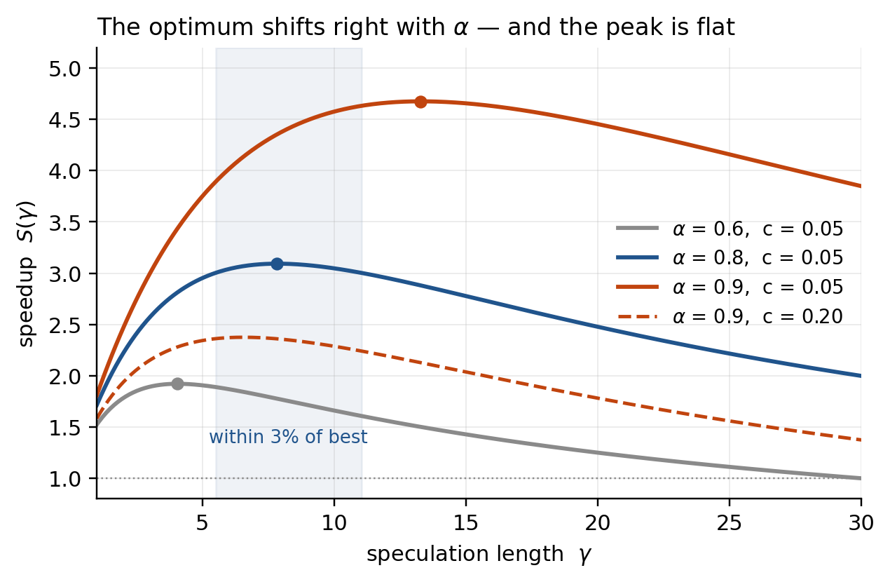
The peak shifts right as $\alpha$ grows. It is also flat: at $\alpha = 0.8$ and $c = 0.05$, every $\gamma$ from 6 to 11 is within 3% of optimal. Getting $\alpha$ and $c$ right matters far more than getting $\gamma$ exactly right, which is why adaptive-$\gamma$ schedulers earn their keep by staying out of the region where $\gamma$ is far too large, not by locating $\gamma^\star$ precisely.

Setting $\partial S / \partial \gamma = 0$ gives the stationarity condition

whose left side is strictly decreasing in $\gamma$, so $S$ is unimodal. Good news for any scheduler that searches $\gamma$ greedily.

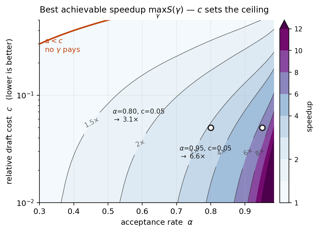
The picture makes the ceiling concrete. Movement along the $\alpha$ axis buys much less than movement down the $c$ axis, and below the $\alpha = c$ line no $\gamma$ helps at all.

How far off the ceiling you actually land is worth internalizing. At $c = 0.05$ the bound is $1/c = 20$, but $\alpha = 0.95$ tops out at $6.6$ (at $\gamma^\star \approx 21$), and $\alpha = 0.8$ at $3.1$. The ceiling is a bound, not a target.

Reallocating $\gamma$: trees instead of chains

One lever deserves a note before we move on. Reallocating $\gamma$ means replacing the scalar with a structure: instead of one chain of $\gamma$ tokens, draft a tree of candidate continuations and verify many chains in a single target pass, under a mask that keeps each branch causal with respect to its own ancestors. The budget is unchanged; only the shape of the spend is.

Choosing that shape has a clean answer. Value each node by its survival probability $a_v$, the chance it is reached and accepted, and take the global top-$n$. Because $a_v$ can only decrease along a root path, that greedy choice is prefix-closed once ties are broken toward the shallower node, and a short induction shows it is optimal at fixed budget. The same argument reappears over three different index sets (tree nodes, draft positions within a block, whole requests in a batch), which is why one proposition ends up covering tree construction, draft-length selection, and batch scheduling alike. It fixes how to spend a budget, not how large the budget should be.

Why speculation spends more compute | the second theorem

$S(\gamma)$ is a wall-clock statement. It assumes the extra verified tokens are free, which holds only in the memory-bound regime.

Leviathan et al. state a second theorem in the same paper, this one counting arithmetic operations rather than wall-clock time. With $\hat{c}$ the drafter's operations ratio, the expected increase in total arithmetic is:

Speculative decoding costs more compute than it saves. It converts compute into latency.

So if you are optimizing time-to-token at fixed load, $S(\gamma)$ is your number and speculation is a win. If you are optimizing tokens per second at saturation, the equation above is your number and speculation is a cost. Both readings are correct. A benchmark that reports only one of them has not told you whether to deploy it.

This shows up in production. DeepSeek's hardware retrospective describes MTP as slightly hurting throughput while significantly improving end-to-end latency. That is the operations-count theorem, observed at scale.

What VESSL AI measured

VESSL AI serves several open-source models, including GLM-5.2 and MiniMax-M3, in production on VESSL Cloud with speculative decoding, and the number that comes back depends less on the drafter than on where it is measured.

Here is one system, Solar-Open2-250B with a DSpark drafter, measured against plain autoregressive decoding at six operating points, three runs each.

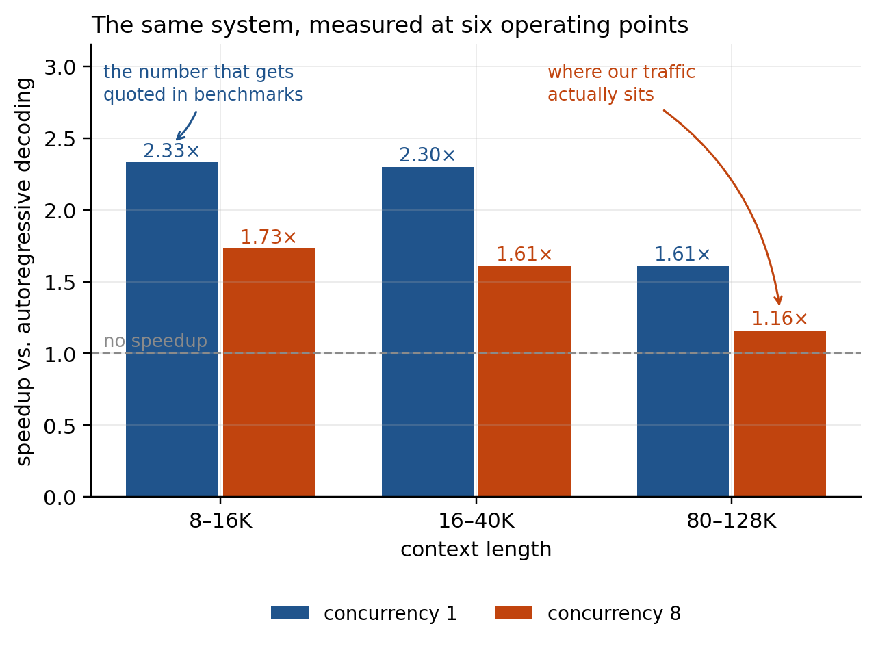
Two axes, and they multiply. Going from concurrency 1 to concurrency 8 costs about 26%. Going from an 8–16K context to an 80–128K one costs about 31%. Together they take 2.33× down to 1.16×.

Nothing about the drafter changed between the top-left cell and the bottom-right one. Both numbers are correct. Only one of them describes a deployment.

The same technique can win big and then lose

On GLM-5.2 with the same drafter family, a single-stream request gets 2.99×, with mean accepted length 4.44, up from 1.93 with the model's built-in MTP head. Raise concurrency to 64 and acceptance holds, but the speedup does not: past some load the extra verification work costs more than the saved passes.

That is the second theorem from earlier in this post, met in production. Speculation spends compute to buy latency. When compute is the scarce resource, there is nothing to buy it with.

The drafter behind these numbers: DSpark

The drafter in the measurements above is DSpark, led by DeepSeek-AI with Peking University collaborators and deployed in DeepSeek's own serving stack; both the Solar-Open2-250B and GLM-5.2 runs use drafters of this family, trained against those targets.

DSpark is a parallel drafter. Instead of producing $\gamma$ tokens one at a time, it fills the whole draft block in a single forward pass, on a backbone it takes from DFlash rather than inventing. Drafting costs one pass, so $c$ drops, and the ceiling $1/c$ from the equation above rises.

The weakness of parallel drafting is that positions cannot see each other. Each position predicts without knowing which token was actually sampled before it, so where the target is torn between several continuations, incoherent combinations appear and acceptance falls. DSpark adds a light sequential correction on top, adjusting each position's logits based on the previous token. The correction costs about as much as an embedding lookup, so $c$ barely moves, while consistency inside the block comes back and $\alpha$ rises.

The last piece is scheduling. DSpark also predicts, for each position, the probability that the draft survives that far, and allocates verification budget across every request in the batch in that order. $\gamma$ stops being a fixed hyperparameter and becomes a per-request value that depends on load. Given how much speedup varies across operating points, in production this piece matters as much as the drafter itself.

Where this leaves us

Speculative decoding is one equation with three parameters and a hard ceiling. Once you know your $\alpha$, your $c$, and the load you actually serve, you can read a new paper's abstract, work out which of the four terms it moves, and estimate what it would buy you before writing any code.

And a speedup quoted without its operating point is not a result. It is one cell of a table.

The open question is how to raise $\alpha$ without paying it all back in $c$. Every drafter architecture is an answer to that, and they differ mainly in what the drafter is allowed to see before it commits to a guess.