Speculative Decoding, Part 2: A History of Drafters

Part 2 of 2. Part 1 covered the governing equation and the four levers.

TL;DR

• The architecture work answers one question: where does the draft's conditioning signal come from?
• The earliest drafters propose in parallel. Increasingly autoregressive ones follow. Then the newest designs return to parallel proposal with a small correction attached.
• Two answers accumulated in between: conditioning should come from features rather than tokens, and letting each position see what was actually sampled before it buys more than it costs.

Intro

Part 1 covered the equation below.

You need a drafter that is both accurate and cheap, and there is a trade-off between the two.

The architecture work answers one question: where does the draft's conditioning signal come from? Conditioning here means what the drafter has to go on when it predicts position $k$. It might see nothing but the trunk's hidden state, or it might take the previous token and run the drafter again, one step at a time.

Every drafter settles two things. What it sees, which sets $\alpha$. How many sequential steps it takes, which sets $c$. The tension is that the cheapest conditioning is the least informative.

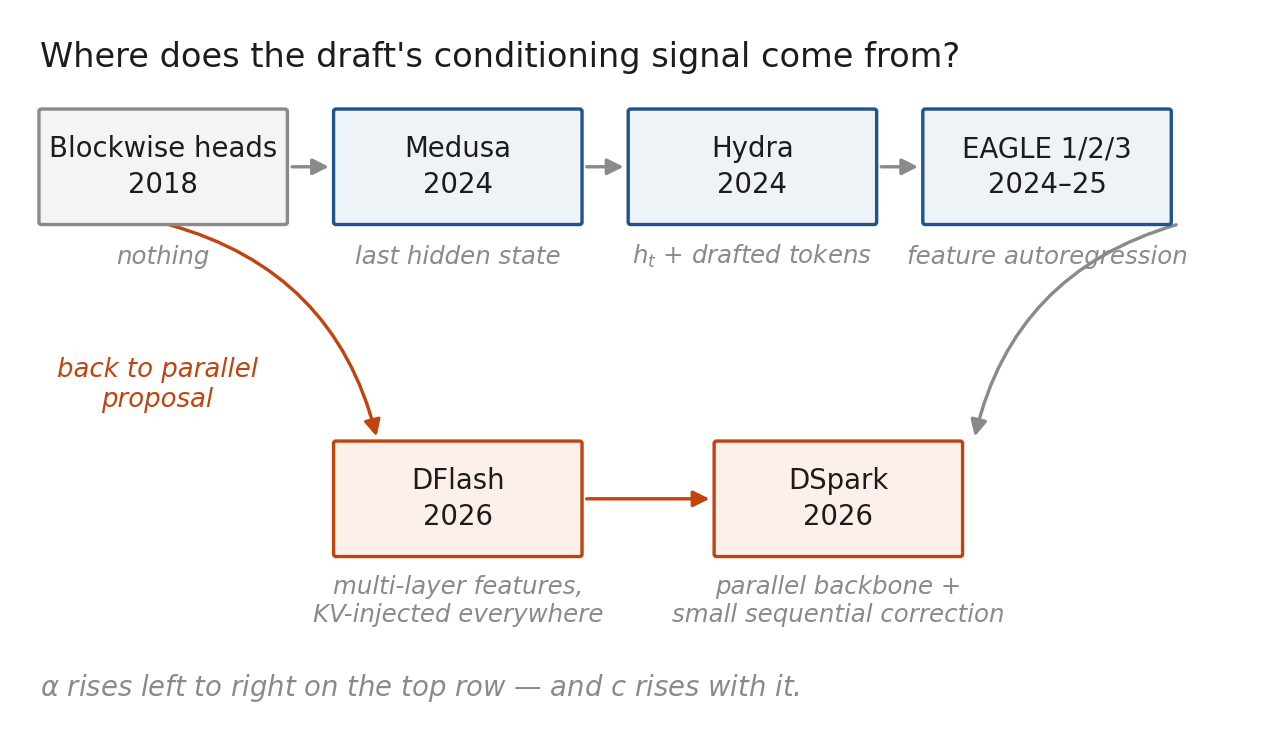
The earliest drafters propose in parallel. Increasingly autoregressive ones follow. Then the newest designs return to parallel proposal with a small correction attached.

Blockwise decoding: the structure, without the conditioning

Blockwise parallel decoding adds $k$ output heads, where head $j$ predicts $x_{t+j}$ from the shared trunk state $h_t$:

Verify in one pass, accept the longest matching prefix. Treat this as the basic structural template for modern speculative decoding. What is missing is any way for the heads to condition on each other: in this structure, head 2 does not know what head 1 produced.

Medusa keeps this structure and works on the heads.

Medusa: heads on the backbone

Medusa attaches $K$ independent heads to the backbone's final hidden state. Each head is one residual FFN block:

Initialize $W_1^{(k)}$ to zero and $W_2^{(k)}$ from a copy of the LM head, and each head starts out reproducing the backbone's own next-token prediction. What gets trained is not a new predictor but the offset from one step ahead to $k$ steps ahead.

The loss is a cross-entropy whose weight decays with position. Head $k$ only gets a turn when every earlier position was accepted, so if head 1 is wrong the draft stops there and whatever the later heads produced no longer matters. The same training budget goes further spent on the early heads.

What that decay rate should be is derivable, and it scales with $\alpha^{k-1}$. The values actually in use did not come from that. Medusa uses $0.8^k$, which its paper calls "a constant like 0.8," and EAGLE-3's public code uses the same 0.8. DFlash picks 7, 5 and 4 to match its block sizes. DSpark ties the decay to block size rather than choosing it separately. None of them sets the rate by looking at $\alpha$, and using a fixed value amounts to assuming $\alpha$ is fixed. Since $\alpha$ varies by domain and shifts from position to position inside a single sentence, a decay rate pinned down at training time may not fit what you serve.

Hydra: buy the joint back, cheaply

Medusa's heads are conditionally independent given $h_t$. Hydra feeds previously drafted tokens' embeddings into the later heads:

But Hydra matters here for a measurement, not an architecture. Its authors trained EAGLE heads on the same base model and found that EAGLE achieves a higher average accepted length, while the two reach comparable throughput.

The Hydra paper attributes this to the cost of EAGLE's draft heads. EAGLE queries a full self-attention block for every position in the candidate continuation. Hydra queries one, once per decoding step. EAGLE buys $\alpha$, Hydra buys $c$, and $S$ ties.

EAGLE: autoregress at the wrong level, on purpose

EAGLE's contribution is a reframing of what the drafter should be predicting.

Token-level autoregression is the wrong level for a small drafter. The token sequence is high-entropy. But the feature sequence is smooth, and one decoder layer can extrapolate it. Those features are the target's second-to-top hidden states, meaning the ones it is about to hand to its LM head. What is left over is which token was actually sampled, and that gets supplied directly:

Note the index shift. The feature at $i$ pairs with the embedding at $i+1$. $f_i$ alone does not determine $f_{i+1}$, because sampling intervened. So the drafter's job becomes extrapolation conditioned on the realized sample, a far easier problem than prediction.

The loss:

Feature regression is the primary term; token prediction carries the 0.1 weight. The order is worth holding onto, because EAGLE-3 drops the primary term outright and keeps only the one that carried 0.1.

EAGLE-2 stops fixing the shape of the draft tree. It scores each branch by multiplying the drafter's confidences along the path from the root, which estimates how likely that branch is to be used at all, and keeps the highest. Because the score is a product along the path, a parent always scores at least as high as its children, so taking the top few pulls the parents in with them.

EAGLE-3 switches from reading only the target's top layer to mixing its low, middle and high layers, and has the drafter take its own output back as input during training. Training on its own output means the predicted feature no longer has to match the real one, and the loss that demanded that match was exactly what pinned the drafter to the top layer.

EAGLE-1 and EAGLE-2 train and serve on different things. In training the drafter is handed the real feature the target produced; at inference it has to carry on from the feature it produced itself, so the longer the draft runs the further it drifts. EAGLE-3 closes that gap by feeding the drafter its own output during training (training-time test), which is why the same size of drafter now sustains a longer draft.

MTP: the drafter moves into pretraining

Multi-token prediction did not start as an inference technique. It is a pretraining objective: rather than predicting the next token, the model predicts the next $n$ at once, and what it was after was quality rather than speed. The gains were largest on code.

Being usable as a drafter followed from that. DeepSeek-V3 chains the modules instead of running parallel heads, so each module takes the previous module's representation together with the token actually sampled at that position. Concatenating a token embedding onto a representation is exactly what EAGLE does. Two different motivations arrived at the same design.

The released config uses depth $D = 1$: a single-layer module, repurposed at serving time as a one-token drafter. Reported second-token acceptance is 85–90%, giving about 1.8× TPS. Put that through Part 1's equation and the drafter cost $c$ lands near 0.04, where one layer out of 61 would be 0.016, two and a half times less. The module does not just run one layer; it also runs the projection over the full vocabulary that turns its state into token probabilities.

But $\alpha$ was fixed during pretraining against a different objective, and the serving side cannot touch it without retraining the model.

DFlash: drafting in parallel

Instead of drawing tokens one at a time, DFlash lays the blanks out side by side and fills them in a single pass. Dropping the mask that hides what comes next lets every position see every other, so drafting costs one forward pass rather than $\gamma$ of them.

What makes this work is KV injection. Hidden states taken from several target layers are projected into the draft's space and inserted into the keys and values that every draft layer attends to, so the drafter sees the target's state throughout its own computation.

The only added parameter is that projection $W_c$, about 42 MB in bf16 against a ~70 GB target, which in memory terms is nothing at all.

Injecting at every layer rather than once at the input has its own reason. Context supplied only at the entrance gets mixed into the draft's own computation and buried as depth grows, so stacking draft layers raises $c$ without raising acceptance. Keep feeding it into every layer's keys and values and the deep layers receive the target's state directly, at which point acceptance scales with depth. That is what lets DFlash run a five-layer draft.

DSpark: putting the joint back

DSpark makes two changes to a parallel backbone.

The first is a small sequential stage. To the backbone's per-position scores it adds a value that depends on which token came immediately before, which makes the positions inside a block depend on one another. Rather than hold that value as a table the size of the vocabulary squared, it is compressed to rank 256, so the whole correction costs $O(r)$ per step.

The second is that deciding how much to verify becomes a scheduling problem. A confidence head predicts, for each position, the probability that it survives given that everything before it was accepted, and the label it is trained against is $\alpha = 1 - D_{TV}$. What was a theorem in Part 1 is a per-token training target here.

Those predictions are then calibrated. A threshold only needs the ranking to be right, but a scheduler that multiplies probabilities into an expected length needs the magnitudes to be right too. Small overestimates compound: at $\gamma = 7$, 10% high at each position leaves the final estimate roughly 95% too high.

The scheduler then takes every request in the batch, hands out verification budget starting from the positions most likely to survive, and maximizes total throughput against a profiled hardware curve. $\gamma$ stops being a number set in advance and becomes something that varies per request and with load.

One ablation captures the trade: a 2-layer DSpark outperforms a 5-layer DFlash. The sequential correction substitutes for depth, not just complements it.

In short

Drafter design started out proposing in parallel, drifted toward autoregression, and came back to parallel. The place it came back to is not the place it left. Two answers accumulated in between: conditioning should come from features rather than tokens, and letting each position see what was actually sampled before it buys more than it costs. The second one in particular was confirmed twice, once when Hydra patched Medusa and again when DSpark patched DFlash.